Data-Driven Snooker Rankings

1. The Data

The data which was scraped from cuetracker is already available on my Github so let’s load this into R straight away. There’ll be two dataframes, one describing every match played over 50 years of the sport and the other describing the details of the different tournaments in the same time period.

## load the packages
options(tidyverse.quiet = TRUE)
library(tidyverse)
library(scales)
library(cowplot)
library(tidygraph)
library(igraph)
library(ggrepel)
library(Matrix)
theme_set(theme_light())

tourn_df <- read_csv('https://raw.githubusercontent.com/obrienjoey/snooker_rankings/master/Data/final_tourn_df.csv')
match_df <- read_csv('https://raw.githubusercontent.com/obrienjoey/snooker_rankings/master/Data/final_match_df.csv')

2. Exploratory Data Analysis

Okay so now we can dive in and do some analysis on these two dataframes using the tidyverse toolbox. First of all how many matches are in the data?

match_df %>%
  select(match_id) %>%
  unique() %>%
  nrow()

## [1] 47710

And what about the actual players?

match_df %>%
  select(match_id, player_1, player_2) %>%
  pivot_longer(2:3, values_to = 'player') %>%
  select(player) %>%
  unique() %>%
  nrow()

## [1] 1221

Lastly how many tournaments were played?

tourn_df %>%
  nrow()

## [1] 657

Okay, that is a good start let’s consider a more technical problem and check which player’s have won the most matches

# find the result frequencies of each player
player_result_df <- match_df %>%
  filter(walkover != TRUE) %>%
  select(match_id, season, player_1, player_2, player_1_score, player_2_score) %>%
  mutate(winner = if_else(player_1_score > player_2_score,
                          player_1, player_2),
         loser = if_else(player_1_score > player_2_score,
                         player_2, player_1)
  ) %>%
  select(match_id, winner, loser) %>%
  pivot_longer(cols = 2:3, values_to = 'player', names_to = 'result') %>%
  group_by(result, player) %>%
  tally() %>%
  ungroup() %>%
  pivot_wider(names_from = 'result', values_from = 'n') %>%
  mutate(loser = replace_na(loser, 0),
         winner = replace_na(winner,0),
         total = loser + winner) %>%
  pivot_longer(cols = 2:4, names_to = 'result',
               values_to = 'matches')


player_result_df %>%
  filter(result == 'winner') %>%
  select(-result) %>%
  arrange(desc(matches)) %>%
  slice(1:5)

## # A tibble: 5 x 2
##   player            matches
##   <chr>               <int>
## 1 John Higgins          899
## 2 Ronnie O'Sullivan     843
## 3 Stephen Hendry        818
## 4 Mark Williams         768
## 5 Steve Davis           761

So there we have the top five ranked players based on the number of wins they have had during their career.

Interestingly, there is also a temporal element to this data in that the matches each occur within a given year, let’s look at how the above values vary over time

# number of tournaments by season
tourn_season_plot <- match_df %>%
  mutate(season = as.integer(season)) %>%
  group_by(season) %>%
  summarise(no_tournaments = n_distinct(tourn_id)) %>%
  ggplot(aes(x = season, y = no_tournaments)) +
  geom_bar(stat='identity', fill = '#008DA8',
           color = 'black') +
  scale_x_continuous(expand = c(0,0), breaks = seq(1968,2020,4)) +
  scale_y_continuous(expand = c(0,0)) +
  theme_minimal() +
  labs(x = 'Season', y = 'Number of Tournaments') +
  theme(axis.line = element_line(),
        axis.text=element_text(size=12),
        plot.title.position = 'plot',
        panel.grid.major.x = element_blank(),
        legend.text=element_text(size=12),
        legend.position = c(0.85,0.9),
        axis.text.x = element_text(angle = 60, hjust = 1),
        plot.title = element_text(size = 14, face = 'bold'),
        axis.title=element_text(size=14))

# number of players by season
player_season_plot <- match_df %>%
  select(season, player_1, player_2) %>%
  pivot_longer(cols = 2:3, values_to = 'player') %>%
  mutate(season = as.integer(season)) %>%
  group_by(season) %>%
  summarise(no_players = n_distinct(player)) %>%
  ggplot(aes(x = season, y = no_players)) +
  geom_bar(stat='identity', fill = '#008DA8',
           color = 'black') +
  theme_minimal() +
  scale_x_continuous(expand = c(0,0), breaks = seq(1968,2020,4)) +
  scale_y_continuous(expand = c(0,0)) +
  labs(x = 'Season', y = 'Number of Players') +
  theme(axis.line = element_line(),
        axis.text=element_text(size=12),
        plot.title.position = 'plot',
        panel.grid.major.x = element_blank(),
        legend.text=element_text(size=12),
        legend.position = c(0.85,0.9),
        axis.text.x = element_text(angle = 60, hjust = 1, size = 10),
        plot.title = element_text(size = 14, face = 'bold'),
        axis.title=element_text(size=14))

cowplot::plot_grid(tourn_season_plot, player_season_plot)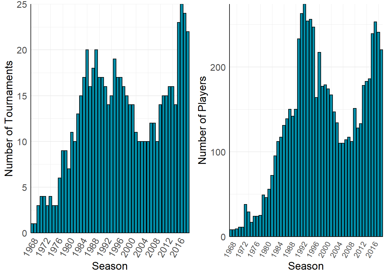

# plot the probability distribution of results obtained by each player
player_result_df %>%
  group_by(result, matches) %>%
  summarise(n = n()) %>%
  ungroup() %>%
  mutate(freq = n / sum(n)) %>%
  filter(matches != 0) %>%
  ggplot(aes(x = matches, y = freq, col = result)) +
  geom_point() +
  scale_y_log10(labels=trans_format('log10',math_format(10^.x))) +
  scale_x_log10(labels=trans_format('log10',math_format(10^.x))) +
  labs(y = 'Probability',
       x = 'Number of Matches'
  ) +
  theme_minimal() +
  scale_color_manual(name = '',
                     breaks = c('total', 'winner', 'loser'),
                     values = c('#008DA8','#C3627D','#4A904D'),
                     labels = c('Total', 'Won', 'Lost')) +
  theme(axis.line = element_line(colour = 'black'),
        axis.text=element_text(size=12),
        plot.title.position = 'plot',
        legend.text=element_text(size=12),
        legend.position = c(0.85,0.85),
        plot.title = element_text(size = 14, face = 'bold'),
        axis.title=element_text(size=14))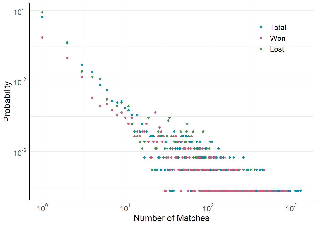

result_df <- match_df %>%
    filter(walkover != TRUE) %>%
    select(match_id, player_1, player_2, player_1_score, player_2_score) %>%
    mutate(winner = if_else(player_1_score > player_2_score,
                            player_1, player_2),
           loser = if_else(player_1_score > player_2_score,
                           player_2, player_1),
    ) %>%
    select(winner, loser)

3. The Model

So now getting to the main aim of this post, let’s borrow some tools from network science to help figuring out an alternative way of ranking snooker players. We’ll use what is known as PageRank, an algorithm originally developed by the founders of Google in ranking webpages that helped their search engine return better results!

The main idea is to represent the sport as a graph, where each of the \(N\) players are a node and the edges of the graph are created by considering the matches played between players. Importantly, the result of the match is important and this is captured by the direction of the edge we draw, so in each match we draw the edge from loser to winner. After consider all matches in the dataset we obtain a \(N \times N\) matrix with entries \(w_{ij}\) describing the number of times player \(i\) has lost to player \(j\).

With this set-up we can proceed to use the PageRank algorithm to rank the players based on the prestige of player \(i\) - \(P_i\), obtained from the following set of equations (feel free to ignore this part if equations aren’t your thing)

\[\begin{equation} P_i = (1-q)\sum_j P_j \frac{w_{ji}}{k_j^{\text{out}}} + \frac{q}{N} + \frac{1-q}{N}\sum_j P_j \delta(k_j^{\text{out}}) \end{equation}\]

Importantly this algorithm considers not only how many times one player defeated another but also how frequently the defeated player themselves defeated others. In this sense each player has some associated prestige describing their quality, and in defeating a player the winner receives some of this associated prestige. This implies that a win against a strong competitor with high prestige is now more worthwhile to a player’s rank than defeating a weaker competitor.

Okay, so no doubt there are plenty of software packages to do this calculation for us but sometimes it is nice to code up the system ourselves so let’s do that now, using the brilliant tidygraph and igraph packages to work with the networks.

page_rank_sim = function(match_result_df){

  node_list <- match_result_df %>%
    gather() %>%
    select(-key) %>%
    unique() %>%
    rename(label = value) %>%
    rowid_to_column("id")

  el <- match_result_df %>%
    count(winner, loser, name = 'weight') %>%
    rename(target = winner,
           source = loser) %>%
    left_join(., node_list, by = c('source' = 'label')) %>%
    rename(from = id) %>%
    left_join(., node_list, by = c('target' = 'label')) %>%
    rename(to = id) %>%
    select(to, from, weight)

  snooker_net <- tbl_graph(nodes = node_list,
                           edges = el,
                           directed = TRUE)
  adj <- as_adj(snooker_net, sparse = TRUE, attr = 'weight')

  ### PageRank algorithm

  N <- node_list %>% nrow() # number of nodes in the network
  P0 <- rep(1/N, N) # initial values
  q = 0.15 # page rank factor
  s_out <- rowSums(adj) # outdegree of the nodes

  P_temp <- P0
  thres <- 1e-20
  error <- 1
  iter = 1
  while(error > thres & iter < 1e4){
    temp <- (1-q)*((P_temp/s_out) %*% adj) + (q/N) + ((1-q)/N)*(P0 * (s_out == 0))
    error <- max(P_temp - temp)
    P_temp <- temp
    iter <- iter + 1
  }

  prestige <- as.vector(temp)

  result <- tibble(player = node_list$label, prestige = prestige,
                   in_strength = as.vector(colSums(adj))) %>%
    arrange(desc(prestige)) %>%
    mutate(rank_pre = rank(-prestige, ties.method = "first"),
           rank_str = rank(-in_strength, ties.method = "first"))

  result
}

4. Results

Using the approach described above, after constructing a network based upon all recorded professional snooker games, it can quickly be determined who is the greatest player of all time. Interestingly, it is not Ronnie O’Sullivan with his natural talent, Steve Davis and his distinguished trophy room, or the winning machine known as Stephen Hendry, but rather the four-time world champion John Higgins! This result may seem surprising to some snooker fans but when the data is considered it is entirely understandable. While both Davis and Hendry have plenty of trophies and wins to their name, the quality of player competing in their era was considerably less than those faced by Higgins and O’Sullivan (who is ranked the second greatest through our approach).

set.seed(1)

# perform the PageRank
all_time_df <- page_rank_sim(result_df)

all_time_df %>%
  filter(rank_pre <= 30 | rank_str <= 30) %>%
  ggplot(aes(x = rank_str, y = rank_pre, label = player)) +
  geom_abline(slope = 1, intercept = 0,
              color="red",
              linetype="dashed", size=1) +
  geom_point() +
  theme_minimal() +
  geom_text_repel(size = 2.25) +
  labs(x = 'Rank by Wins',
       y = 'Rank by PageRank') +
  theme(axis.line = element_line(colour = 'black'),
        axis.text=element_text(size=10),
        plot.title.position = 'plot',
        plot.title = element_text(size = 14, face = 'bold'),
        plot.subtitle = element_text(size = 12),
        axis.title=element_text(size=12))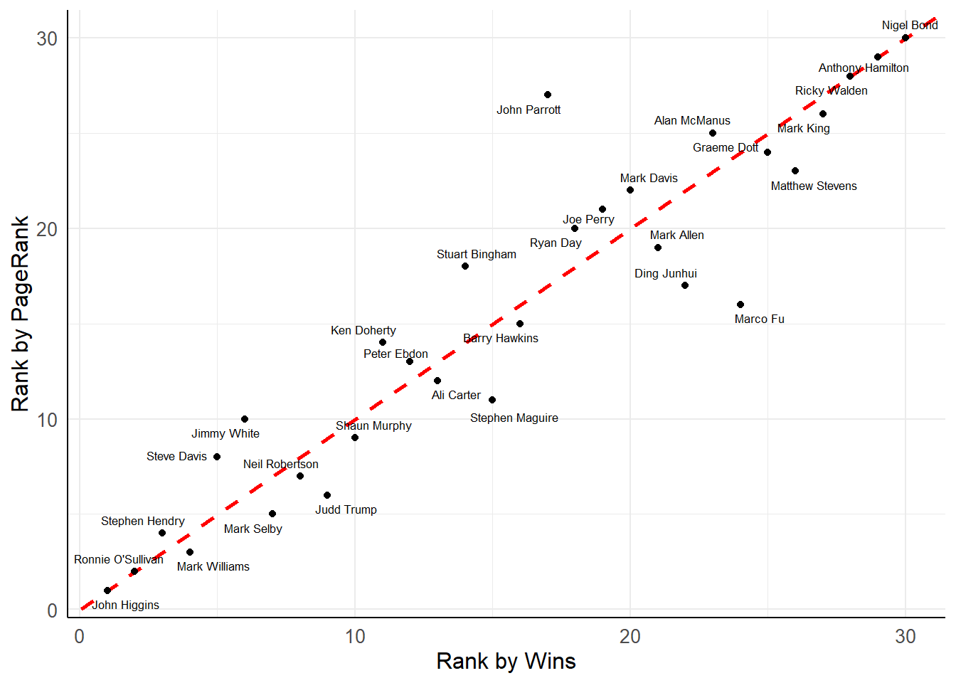

5. Concluding Thoughts

In order to help satisfy the intrinsic human desire to rank entities, this work has proposed a method which utilizes a mathematical framework to determine a ranking of competitors which considers not only the number of times a player has won but also the quality associated with each win.