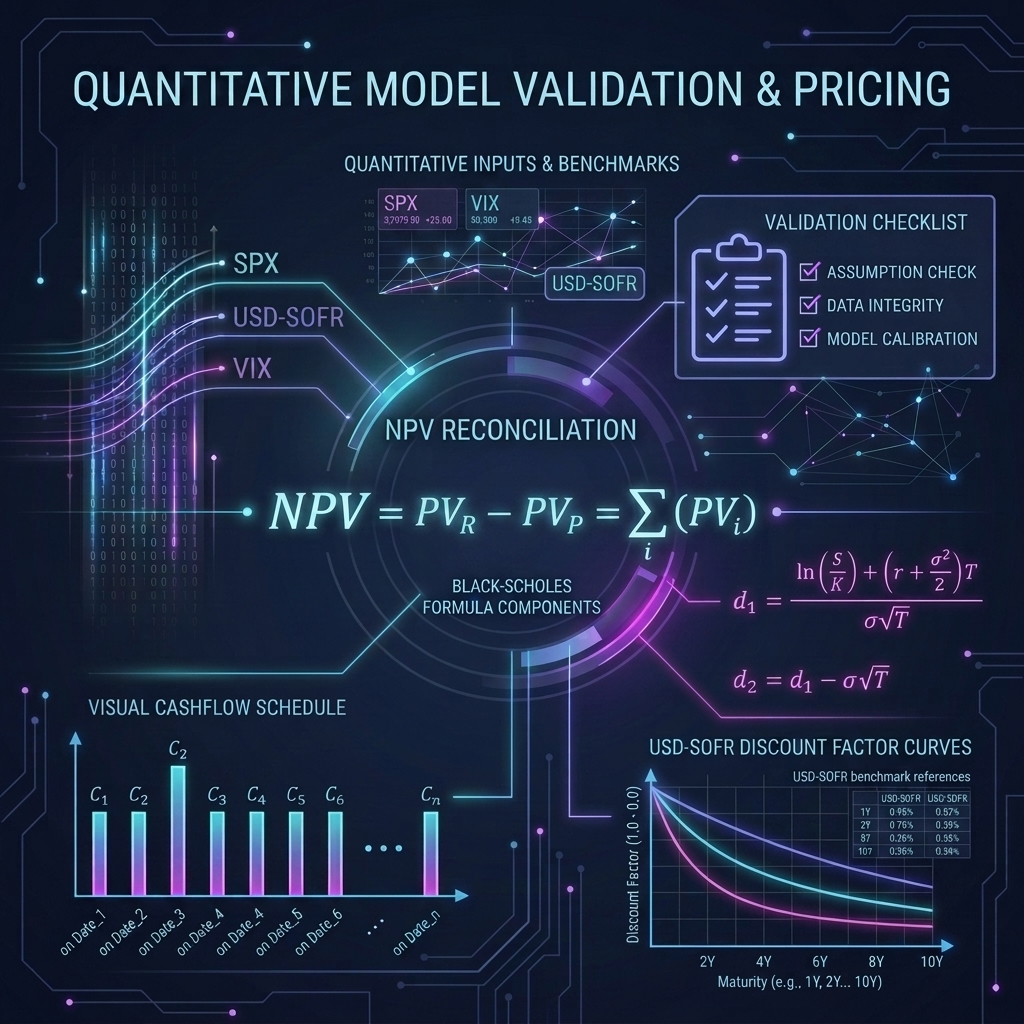
One of the most important, and frequently underestimated, challenges when adopting a quantitative risk library is model validation. Whether you are evaluating a new engine against an incumbent system, or maintaining an already-live implementation, you need to be able to answer a deceptively hard question: does this number make sense?
With most commercial black-box pricing libraries, this is genuinely difficult. You receive a single aggregated NPV with little visibility into the discount factors applied, the forward rates projected, or the internal model parameters used. When numbers diverge, debugging can become an exercise in reverse-engineering an opaque system.
Open Source Risk Engine (ORE) takes a different approach. Because the source code is fully available and the output is deliberately structured and transparent, ORE exposes everything you need to audit a result from first principles, with two complementary pathways in particular:
- The Cashflow Report (
flows.csv) — a payment-by-payment audit trail that lets you reconstruct any trade’s NPV by hand from raw cashflow amounts and discount factors. - The Additional Results File (
additional_results.csv) — a per-trade diagnostic surfacing every internal model parameter used in pricing, making it possible to back out the exact formula applied.
Both are demonstrated here using two trade types: the Interest Rate Swap and the European Equity Option.
When is this useful?
There are two common validation contexts in which this workflow applies:
- Validating ORE itself: You are benchmarking ORE’s output against a theoretical model or an existing system. Cashflow-level transparency lets you trace any discrepancy to a specific convention difference or curve configuration.
- Using ORE as a validation library: You are treating ORE as your reference implementation and verifying that trade results from another system reconcile to it.
In either case, the ability to back out every intermediate value, without needing source code access or vendor cooperation, is what makes ORE well suited to this role.
1. The Validation Framework — ore.xml
Both validation pathways require specific analytics to be enabled in ORE’s master configuration file (ore.xml). The examples enable the NPV report with additionalResults, the cashflow report, and the curve export analytic used for the optional forward-rate check:
<Analytics>
    <Analytic type="npv">
        <Parameter name="active">Y</Parameter>
        <Parameter name="baseCurrency">EUR</Parameter>
        <Parameter name="outputFileName">npv.csv</Parameter>
        <Parameter name="additionalResults">Y</Parameter>
        <Parameter name="additionalResultsReportPrecision">12</Parameter>
    </Analytic>
    <Analytic type="cashflow">
        <Parameter name="active">Y</Parameter>
        <Parameter name="outputFileName">flows.csv</Parameter>
    </Analytic>
    <Analytic type="curves">
        <Parameter name="active">Y</Parameter>
        <Parameter name="configuration">default</Parameter>
        <Parameter name="grid">7300,1D</Parameter>
        <Parameter name="outputFileName">curves.csv</Parameter>
    </Analytic>
</Analytics>
The critical flag here is <Parameter name="additionalResults">Y</Parameter>. When enabled, ORE writes a companion file (additional_results.csv) containing all the raw model inputs and intermediate quantities computed during pricing. This enables the second validation pathway, covered in Section 3. The <Parameter name="additionalResultsReportPrecision">12</Parameter> value controls how many decimal places ORE writes for the numeric results in that file.
2. Validation Pathway 1: The Cashflow Report — EUR Interest Rate Swap
2.1 Trade Configuration — portfolio.xml
Our first example is a 20-year EUR Interest Rate Swap (Swap_20y), valued as of 2025-02-10, starting on 2023-02-21 and maturing on 2043-02-21. We receive a fixed rate of 2.1% annually and pay 6M EURIBOR semi-annually on a notional of €10,000,000.
<Portfolio>
    <Trade id="Swap_20y">
        <TradeType>Swap</TradeType>
        <Envelope>
            <CounterParty>CPTY</CounterParty>
            <NettingSetId>NS</NettingSetId>
        </Envelope>
        <SwapData>
            <LegData>
                <LegType>Fixed</LegType>
                <Payer>false</Payer>
                <Currency>EUR</Currency>
                <Notionals>
                    <Notional>10000000</Notional>
                </Notionals>
                <DayCounter>A360</DayCounter>
                <PaymentConvention>MF</PaymentConvention>
                <FixedLegData>
                    <Rates>
                        <Rate>0.021</Rate>
                    </Rates>
                </FixedLegData>
                <ScheduleData>
                    <Rules>
                        <StartDate>2023-02-21</StartDate>
                        <EndDate>2043-02-21</EndDate>
                        <Tenor>1Y</Tenor>
                        <Calendar>TARGET</Calendar>
                        <Convention>MF</Convention>
                        <Rule>Forward</Rule>
                    </Rules>
                </ScheduleData>
            </LegData>
            <LegData>
                <LegType>Floating</LegType>
                <Payer>true</Payer>
                <Currency>EUR</Currency>
                <Notionals>
                    <Notional>10000000</Notional>
                </Notionals>
                <DayCounter>A360</DayCounter>
                <PaymentConvention>MF</PaymentConvention>
                <FloatingLegData>
                    <Index>EUR-EURIBOR-6M</Index>
                    <Spreads>
                        <Spread>0.000000</Spread>
                    </Spreads>
                    <IsInArrears>false</IsInArrears>
                    <FixingDays>2</FixingDays>
                </FloatingLegData>
                <ScheduleData>
                    <Rules>
                        <StartDate>2023-02-21</StartDate>
                        <EndDate>2043-02-21</EndDate>
                        <Tenor>6M</Tenor>
                        <Calendar>TARGET</Calendar>
                        <Convention>MF</Convention>
                        <Rule>Forward</Rule>
                    </Rules>
                </ScheduleData>
            </LegData>
        </SwapData>
    </Trade>
</Portfolio>
Key parameters:
Payer:falseon the Fixed Leg (we receive the 2.1% coupon) andtrueon the Floating Leg (we pay 6M EURIBOR).DayCounter: Both legs useA360(Actual/360).PaymentConvention:MF(Modified Following).Tenor: Fixed leg pays annually (1Y); floating leg resets and pays semi-annually (6M).Calendar:TARGETfor EUR transactions.
2.2 Running the Valuation
The supplied ore.xml sets the as-of date to 2025-02-10 (<Parameter name="asofDate">2025-02-10</Parameter>), and the input and output directories are already wired up. Running ORE is just:
import ORE as ore

params = ore.Parameters()
params.fromFile("Input/ore.xml")
ore.OREApp(params).run()
This generates two primary outputs in the Output directory:
npv.csv: The headline NPV per trade — the figure we are about to reconstruct.flows.csv: A granular breakdown of every scheduled cashflow, including payment dates, accrual fractions, projected rates, discount factors, and individual present values.
Here is what a few rows of flows.csv actually look like (only the columns used in the reconciliation below are shown; the real file also carries currency, accrued-amount, fixing-date, and notional fields):
| LegNo | PayDate | FlowType | Amount (EUR) | Coupon | Accrual | fixingValue | DiscountFactor | PresentValue (EUR) |
|---|---|---|---|---|---|---|---|---|
| 0 | 2025-02-21 | Interest | 213,500.00 | 0.0210000000 | 1.0166666667 | #N/A | 0.9991628390 | 213,321.27 |
| 1 | 2025-02-21 | Interest | -174,186.67 | 0.0340800000 | 0.5111111111 | 0.0340800000 | 0.9991628390 | -174,040.84 |
| 1 | 2025-08-21 | InterestProjected | -121,718.73 | 0.0242092506 | 0.5027777778 | 0.0242092506 | 0.9876472785 | -120,215.17 |
Key columns worth knowing about:
LegNo— 0 is the fixed leg, 1 the floating leg. This is how the script below splits the position.Amount— the actual cashflow amount, signed by direction: positive on the received fixed leg, negative on the paid floating leg.Coupon— the fixed rate (leg 0) or the projected/fixed floating rate (leg 1).fixingValue— the rate actually fixed or projected for floating-leg coupons (shown as#N/Aon the fixed leg).Accrual— the day-count fraction applied to the notional.DiscountFactor— ORE’s discount factor from the valuation date to the payment date.PresentValue— the discounted cashflow, i.e.Amount × DiscountFactor.
Notice the two 2025-02-21 rows: the fixed leg pays a positive 213,500.00 and the floating leg pays a negative -174,186.67 on the same date, each discounted by the same factor 0.9991628390. The third row shows a projected floating coupon (InterestProjected type) for 2025-08-21 — we will verify how that projected rate is derived in Section 2.4.
The NPV report for Swap_20y reads:
| #TradeId | TradeType | NPV (EUR) | NpvCurrency |
|---|---|---|---|
| Swap_20y | Swap | -236,453.7496 | EUR |
That -€236,453.75 is the figure we will now reconstruct line-by-line from flows.csv.
2.3 The Validation Logic
The cashflow report is the first and most direct validation tool. The mathematical principle is relatively simple: the net NPV of a swap position must equal the sum of the present values of all received cashflows minus the sum of the present values of all paid cashflows:
Where for each individual cashflow $i$:
$$\text{PV}_i = \text{Amount}_i \times \text{Discount Factor}_i$$
Note: In ORE’s flows.csv, cashflows on pay legs are signed negatively, so summing PresentValue directly across all leg rows computes this net difference automatically.
Because ORE outputs the resolved DiscountFactor on the payment date for every single flow in flows.csv, we can load the file using pandas and reconstruct this calculation entirely from ORE’s own outputs:
import pandas as pd

def reconcile_pricing():
    flows_df = pd.read_csv("Output/flows.csv")
    npv_df = pd.read_csv("Output/npv.csv")

    flows_df.columns = [c.strip() for c in flows_df.columns]
    npv_df.columns = [c.strip() for c in npv_df.columns]

    # Manual PV = Amount * DiscountFactor
    flows_df["ManualPresentValue"] = flows_df["Amount"] * flows_df["DiscountFactor"]

    # Verify manual PV matches ORE's reported PresentValue column
    max_pv_diff = (flows_df["ManualPresentValue"] - flows_df["PresentValue"]).abs().max()
    print(f"Max difference (Manual vs ORE Flow PV): {max_pv_diff:.2e} EUR")

    # Breakdown by Leg (Leg 0 = Fixed / receive, Leg 1 = Floating / pay)
    leg_names = {0: "Fixed (receive)", 1: "Floating (pay)"}
    leg_groups = flows_df.groupby("LegNo")
    print("\n=== Cashflow Leg Breakdown ===")
    leg_pvs = {}
    for leg_no, group in leg_groups:
        leg_pv = group["PresentValue"].sum()
        leg_pvs[leg_no] = leg_pv
        print(f"Leg {leg_no} ({leg_names.get(leg_no, '?')}) Total PV: {leg_pv:,.4f} EUR")

    reconstructed_npv = flows_df["PresentValue"].sum()
    swap_row = npv_df[npv_df["#TradeId"] == "Swap_20y"]
    reported_npv = swap_row["NPV"].iloc[0]

    print("\n=== PV Reconciliation Summary ===")
    print(f"Reconstructed Net PV:     {reconstructed_npv:,.4f} EUR")
    print(f"ORE Reported NPV:         {reported_npv:,.4f} EUR")
    print(f"Residual Difference:      {reconstructed_npv - reported_npv:.2e} EUR")

    tol = 1e-4  # EUR
    assert abs(reconstructed_npv - reported_npv) < tol, (
        f"Reconciliation failed: residual {abs(reconstructed_npv - reported_npv):.2e} exceeds tolerance {tol:.0e} EUR"
    )
    print(f"Reconciliation passed  (tolerance {tol:.0e} EUR)")

if __name__ == "__main__":
    reconcile_pricing()
Running this produces:
Max difference (Manual vs ORE Flow PV): 4.72e-05 EUR

=== Cashflow Leg Breakdown ===
Leg 0 (Fixed / receive) Total PV: 3,314,499.2500 EUR
Leg 1 (Floating / pay) Total PV: -3,550,952.9996 EUR

=== PV Reconciliation Summary ===
Reconstructed Net PV:     -236,453.7496 EUR
ORE Reported NPV:         -236,453.7496 EUR
Residual Difference:      -1.23e-07 EUR
Reconciliation passed  (tolerance 1e-04 EUR)
Zero residual to machine tolerance. The discount factors embedded in flows.csv are fully consistent with the NPV engine, and if a discrepancy ever appeared, you would have a line-by-line audit trail pointing to exactly which cashflow and which discount factor was off. That level of traceability is not available in a closed system. If one wanted to avoid this Python layer of interaction with the flows report, they can interact directly with the csv spreadsheet to obtain the same result.
Note: the per-flow Max difference (Manual vs ORE Flow PV) of 4.72e-05 EUR is larger than the final Residual Difference of -1.23e-07 EUR. That is expected, ORE writes flows.csv with the Amount column rounded to 4 decimal places, while internally it is using machine precision.
2.4 Digging Deeper: Forward Rate Projection
While the cashflow reconciliation confirms the discounting mechanics, a deeper validation question remains: how are the projected floating rates derived?
For the floating leg (EUR-EURIBOR-6M), future coupons are determined by the forward curve. The forward rate $F$ between two dates $t_{\text{start}}$ and $t_{\text{end}}$ is:
$$F = \frac{1}{\tau} \left( \frac{P(t_0, t_{\text{start}})}{P(t_0, t_{\text{end}})} - 1 \right)$$
Where $P(t_0, t)$ is the discount factor from today to date $t$ on the EUR-EURIBOR-6M forward curve, and $\tau$ is the Actual/360 day count fraction.
The grid setting is configurable. The example uses <Parameter name="grid">7300,1D</Parameter>, which requests 7,300 pillars at daily spacing, with daily dates advanced to working days, more than enough to cover the swap’s 2043 maturity. You could use a smaller or larger number of pillars, or a different spacing such as 120,1M for 120 monthly pillars. Choose a grid that includes the dates you need: a coarser grid may not contain the exact coupon dates used below. ORE writes the resulting discount factors for all configured curves to curves.csv, which we can read with pandas to extract $P(t_0, t_{\text{start}})$ and $P(t_0, t_{\text{end}})$ and back out the exact projected rate:
import pandas as pd
import ORE as ore

def reconcile_floating_rate_from_curves():
    curves_df = pd.read_csv("Output/curves.csv")
    curves_df.columns = [c.strip() for c in curves_df.columns]

    # Select the EUR-EURIBOR-6M column from ORE's wide curves report
    fwd_curve = curves_df[["Date", "EUR_EURIBOR_6M_DF"]]

    # First projected coupon after valuation date (2025-02-10)
    start_date = ore.Date(21, 2, 2025)
    end_date   = ore.Date(21, 8, 2025)

    df_start = fwd_curve[fwd_curve["Date"] == "2025-02-21"]["EUR_EURIBOR_6M_DF"].iloc[0]
    df_end   = fwd_curve[fwd_curve["Date"] == "2025-08-21"]["EUR_EURIBOR_6M_DF"].iloc[0]

    # Compute exact day count and year fraction using ORE's Actual360 day counter
    dc = ore.Actual360()
    days = dc.dayCount(start_date, end_date)      # 181 days
    tau = dc.yearFraction(start_date, end_date)   # 181 / 360 = 0.5027777778

    manual_fwd_rate = (df_start / df_end - 1.0) / tau
    notional = 10_000_000.00
    manual_amount = -1.0 * notional * manual_fwd_rate * tau

    print("\n=== Floating Rate Manual Projection (from curves.csv) ===")
    print(f"Start Date ({start_date.ISO()}) DF: {df_start:.10f}")
    print(f"End Date   ({end_date.ISO()}) DF: {df_end:.10f}")
    print(f"Day Count (Actual/360):      {days} days")
    print(f"Year Fraction (tau):         {tau:.10f}")
    print("-" * 55)
    print(f"Calculated Rate:             {manual_fwd_rate*100:.8f}%")
    print(f"Calculated Flow:             {manual_amount:,.4f} EUR")

if __name__ == "__main__":
    reconcile_floating_rate_from_curves()
=== Floating Rate Manual Projection (from curves.csv) ===
Start Date (2025-02-21) DF: 0.9992545136
End Date   (2025-08-21) DF: 0.9872379781
Day Count (Actual/360):      181 days
Year Fraction (tau):         0.5027777778
------------------------------------------------------
Calculated Rate:             2.42092506%
Calculated Flow:             -121,718.7320 EUR
Comparing this to flows.csv:
- ORE Reported Rate:
2.42092506% - ORE Reported Flow:
-121,718.73 EUR
The numbers agree exactly. The projected rate in flows.csv is derived from the same discount factors pulled from the market object which we can verify directly as above.
3. Validation Pathway 2: The Additional Results File — Equity Option
The cashflow report works well for instruments where the valuation is a sum of discounted cashflows. But for options and other non-linear payoffs, there is typically no cashflow schedule to reconcile against in the same way. Instead, ORE exposes a second validation pathway: the additional_results.csv file.
When additionalResults is enabled, ORE writes every internal pricing parameter used for each trade into this file. For model validation, this means you can take the exact inputs ORE used and reconstruct the pricing formula yourself, verifying that the output is consistent with the closed-form expression.
The option inputs used in this section come from the companion trade translation bundle, configured with the 2023-01-31 as-of date, which we reuse here. The resulting option outputs are included in this post’s bundle in a dedicated Output_Eq directory, kept separate from the swap’s Output/ directory so that re-running the swap’s run_pricing.py never overwrites them.
3.1 The Equity Option Portfolio
From our trade translation adaptor post, we take the long call option on the S&P 500 (RIC:.SPX), valued as of 2023-01-31. This example uses a separate ore.xml setup from the swap example, with matching market data and as-of-date settings:
| TradeID | Type | LongShort | Strike | Quantity | Expiry |
|---|---|---|---|---|---|
EQ_CALL_SP5_1 | Call | Long | 4000.0 | 100 | 2023-07-31 |
The call trade in the full ORE portfolio looks like this:
<Portfolio>
  <Trade id="EQ_CALL_SP5_1">
    <TradeType>EquityOption</TradeType>
    <Envelope>
      <CounterParty>CPTY_A</CounterParty>
    </Envelope>
    <EquityOptionData>
      <OptionData>
        <LongShort>Long</LongShort>
        <OptionType>Call</OptionType>
        <Style>European</Style>
        <ExerciseDates>
          <ExerciseDate>2023-07-31</ExerciseDate>
        </ExerciseDates>
        <Settlement>Cash</Settlement>
        <PremiumAmount>150</PremiumAmount>
        <PremiumCurrency>USD</PremiumCurrency>
        <PremiumPayDate>2023-02-02</PremiumPayDate>
      </OptionData>
      <Underlying>
        <Type>Equity</Type>
        <Name>RIC:.SPX</Name>
      </Underlying>
      <Currency>USD</Currency>
      <Quantity>100</Quantity>
      <Strike>4000</Strike>
    </EquityOptionData>
  </Trade>
</Portfolio>
ORE prices the trade using the analytical Black-Scholes-Merton model (as configured in pricingengine.xml), whose AnalyticEuropeanEngine evaluates the payoff via the Black-76 forward formulation — written in terms of the forward price rather than the spot price (Section 3.3). The NPV run produces:
| #TradeId | TradeType | NPV (USD) | NpvCurrency |
|---|---|---|---|
| EQ_CALL_SP5_1 | EquityOption | 10,818.438615 | USD |
3.2 Reading the Additional Results
The additional_results.csv file captures the raw model parameters used by ORE’s analytic engine for each trade. For EQ_CALL_SP5_1, the relevant rows from the actual ORE run look like this:
| #TradeId | ResultId | ResultType | ResultValue |
|---|---|---|---|
| EQ_CALL_SP5_1 | quantity | double | 100.0000000000000000 |
| EQ_CALL_SP5_1 | strike | double | 4000.0000000000000000 |
| EQ_CALL_SP5_1 | cashFlowResults[0] | cashflows | 112.3500281083220216 @ 2023-07-31 |
| EQ_CALL_SP5_1 | discountFactor | double | 0.9762704874971966 |
| EQ_CALL_SP5_1 | dividendDiscount | double | 0.9762704874971967 |
| EQ_CALL_SP5_1 | forward | double | 4000.0000000000004547 |
| EQ_CALL_SP5_1 | riskFreeDiscount | double | 0.9762704874971966 |
| EQ_CALL_SP5_1 | spot | double | 4000.0000000000000000 |
| EQ_CALL_SP5_1 | timeToExpiry | double | 0.4958904109589041 |
| EQ_CALL_SP5_1 | volatility | double | 0.1000000000000000 |
| _EQ_CALL_SP5_1_1 | premiumAmount | double | 150.0000000000000000 |
| _EQ_CALL_SP5_1_1 | premiumDate | date | 2023-02-02 |
| _EQ_CALL_SP5_1_1 | premiumDiscountFactor | double | 0.9997537072850695 |
ORE reports the forward and discount factors directly, so we can reconstruct the price without converting them back into continuously compounded rates. The premium appears as a separate synthetic cashflow record because PremiumAmount is an absolute amount, not a per-contract amount.
Two small observations before we plug numbers in:
cashFlowResults[0]is the undiscounted payoff:112.350028is ORE’s per-unit payoff at expiry — precisely $F \cdot N(d_1) - K \cdot N(d_2)$ before discounting. Discount it with the reported factor and you get112.350028 × 0.9762704875 = 109.684017— which is exactly the Black-76 value we reconstruct in Section 3.3.timeToExpiry= 0.4958904109589041: that is181 / 365, i.e. the Actual/365 day-count fraction from the valuation date2023-01-31to expiry2023-07-31.
3.3 Reconstructing the Black-76 Formula from Additional Results
While ORE’s AnalyticEuropeanEngine is configured with the BlackScholesMerton model, the closed-form price is evaluated in the Black-76 forward variation of the model here, written in terms of the forward price $F$ rather than the spot price $S$:
$$C = D \cdot \left( F \cdot N(d_1) - K \cdot N(d_2) \right)$$
with
$$d_1 = \frac{\ln(F/K) + \frac{1}{2}\sigma^2 T}{\sigma \sqrt{T}}, \quad d_2 = d_1 - \sigma\sqrt{T}$$
Here $F$ is the forward price, $K$ the strike, $D = e^{-rT}$ the risk-free discount factor, $T$ the time to expiry, and $\sigma$ the volatility. The spot-based BSM formula is mathematically equivalent via the carry relationship $F = S e^{(r-q)T}$, but ORE reports forward, strike, timeToExpiry, volatility, and riskFreeDiscount directly — exactly the inputs the Black-76 formula needs, so we can price without converting anything back into continuously compounded rates.
Plugging the values from additional_results.csv directly into the formula:
import math
import pandas as pd

def black76_validate():
    additional_results_df = pd.read_csv("Output_Eq/additional_results.csv")
    npv = pd.read_csv("Output_Eq/npv.csv")
    additional_results_df.columns = additional_results_df.columns.str.strip()
    npv.columns = npv.columns.str.strip()

    def get_param(trade_id, result_id):
        row = additional_results_df[
            (additional_results_df["#TradeId"] == trade_id) & (additional_results_df["ResultId"] == result_id)
        ]
        return float(row["ResultValue"].iloc[0])

    trade_id = "EQ_CALL_SP5_1"
    premium_id = f"_{trade_id}_1"

    quantity = get_param(trade_id, "quantity")
    F = get_param(trade_id, "forward")
    K = get_param(trade_id, "strike")
    T = get_param(trade_id, "timeToExpiry")
    vol = get_param(trade_id, "volatility")
    discount = get_param(trade_id, "riskFreeDiscount")
    premium_paid = get_param(premium_id, "premiumAmount")
    premium_df = get_param(premium_id, "premiumDiscountFactor")
    ore_npv = npv.loc[npv["#TradeId"] == trade_id, "NPV"].iloc[0]

    print(f"\n=== Additional Results Parameters for {trade_id} ===")
    print(f"  Forward (F):          {F:.6f}")
    print(f"  Strike (K):           {K:.6f}")
    print(f"  Time to Expiry (T):   {T:.10f}")
    print(f"  Volatility:           {vol:.6f}  ({vol*100:.2f}%)")
    print(f"  Risk-Free Discount:   {discount:.10f}  (D = e^(-rT))")

    sqrt_t = math.sqrt(T)
    d1 = (math.log(F / K) + 0.5 * vol**2 * T) / (vol * sqrt_t)
    d2 = d1 - vol * sqrt_t

    print("\n=== d1 / d2 Verification ===")
    print(f"  d1:                     {d1:.10f}")
    print(f"  d2:                     {d2:.10f}")

    normal_cdf = lambda x: (1.0 + math.erf(x / math.sqrt(2.0))) / 2.0
    black76_call = discount * (F * normal_cdf(d1) - K * normal_cdf(d2))
    ore_unit_value = (ore_npv + premium_paid * premium_df) / quantity

    print("\n=== Black-76 Reconstruction ===")
    print(f"  Black-76 Call (manual): {black76_call:.6f} USD  per unit")
    print(f"  ORE Implied Value:      {ore_unit_value:.6f} USD  per unit")
    print(f"  Difference:            {abs(black76_call - ore_unit_value):.2e} USD")

    premium_pv = premium_paid * premium_df
    full_npv_manual = quantity * black76_call - premium_pv

    print("\n=== Full Position NPV Reconciliation ===")
    print(f"  Quantity:             {quantity:.0f} contracts")
    print(f"  Black-76 value per unit: {black76_call:.6f} USD")
    print(f"  Premium amount:        {premium_paid:.2f} USD (PV = {premium_pv:.6f})")
    print(f"  Manual NPV:           {full_npv_manual:,.4f} USD")
    print(f"  ORE Reported NPV:     {ore_npv:,.4f} USD")
    print(f"  Residual:             {abs(full_npv_manual - ore_npv):.4f} USD")

if __name__ == "__main__":
    black76_validate()
Running this gives:
=== Additional Results Parameters for EQ_CALL_SP5_1 ===
  Forward (F):          4000.000000
  Strike (K):           4000.000000
  Time to Expiry (T):   0.4958904110
  Volatility:           0.100000  (10.00%)
  Risk-Free Discount:   0.9762704875  (D = e^(-rT))

=== d1 / d2 Verification ===
  d1:                     0.0352097434
  d2:                     -0.0352097434

=== Black-76 Reconstruction ===
  Black-76 Call (manual): 109.684017 USD  per unit
  ORE Implied Value:      109.684017 USD  per unit
  Difference:             7.08e-10 USD

=== Full Position NPV Reconciliation ===
  Quantity:             100 contracts
  Black-76 value per unit: 109.684017 USD
  Premium amount:        150.00 USD (PV = 149.963056)
  Manual NPV:           10,818.4386 USD
  ORE Reported NPV:     10,818.4386 USD
  Residual:             0.0000 USD
The manual reconstruction agrees with ORE output to machine precision. The forward price, strike, time to expiry, volatility, and the risk-free discount factor all come directly from additional_results.csv, while the premium is taken from its separate synthetic cashflow record. These reports allows one to not have to trust the ORE C++ source blindly: the reported inputs reproduce the final NPV.
A Note on Why $F = S$ (and hence $r = q$)
You may notice that ORE reports forward = 4000, identical to the spot price, and consequently dividendDiscount = riskFreeDiscount. This is not a coincidence or a quirk of ORE — it follows directly from the market data supplied for this example. In the companion trade translation bundle, the S&P 500 equity curve is configured with a spot price of 4000 and a 6M forward price of 4000:
EQUITY/PRICE/RIC:.SPX/USD 4000.00
EQUITY_FWD/PRICE/RIC:.SPX/USD/6M 4000.00
For any forward price, the carry relationship is $F = S \cdot e^{(r-q)T}$. With $F = S$, the exponent must vanish, so $r - q = 0$, i.e., the dividend yield exactly offsets the risk-free rate. Because Black-76 prices in terms of $F$, that carry information enters the formula directly through the reported forward, which is precisely why forward equals spot and dividendDiscount equals riskFreeDiscount in this example. In a real market setup with a forward price different from spot (e.g. a dividend-paying index where the forward trades below spot), $F < S$, $q > r$, and the two discount factors would diverge accordingly, with the reported forward carrying that divergence into the price.
4. Summary
Two complementary pathways cover the main classes of instrument ORE prices:
| Pathway | Output File | Best for |
|---|---|---|
| Cashflow Report | flows.csv | Linear payoffs: swaps, bonds, FRAs. Reconstruct NPV from $\text{PV}_i = \text{Amount}_i \times \text{DF}_i$. |
| Additional Results | additional_results.csv | Non-linear payoffs: options, exotics. Back out model parameters and verify the closed-form formula directly. |
Between them, you are not limited to checking a headline number against a benchmark. You can trace any discrepancy to a specific coupon, a specific discount factor, or a specific model input, details that are rarely surfaced in commercial libraries, and one of the main reasons ORE makes a credible independent validation reference.
Source Code
The swap configuration and reconciliation scripts are available here. The option outputs used in Section 3 are included in the same bundle under Output_Eq, and the option input files and run script that generate them are available in the companion trade translation bundle. The reconcile_option.py script reads from Output_Eq.
Need Help with ORE Integration?
Dropping a risk engine into an established data landscape is rarely plug-and-play. Bespoke trade representations, legacy databases, and user-specific market conventions all get in the way of a clean feed.
If you are evaluating ORE for your team, or need a custom trade translation layer, reach out. We build robust ORE integration layers, market data connectors, and validation pipelines tailored to your stack.

Joey O'Brien
Principal Consultant
Principal Consultant in the Quant Services division of LSEG, specializing in model validation, derivative pricing, and risk solutions.