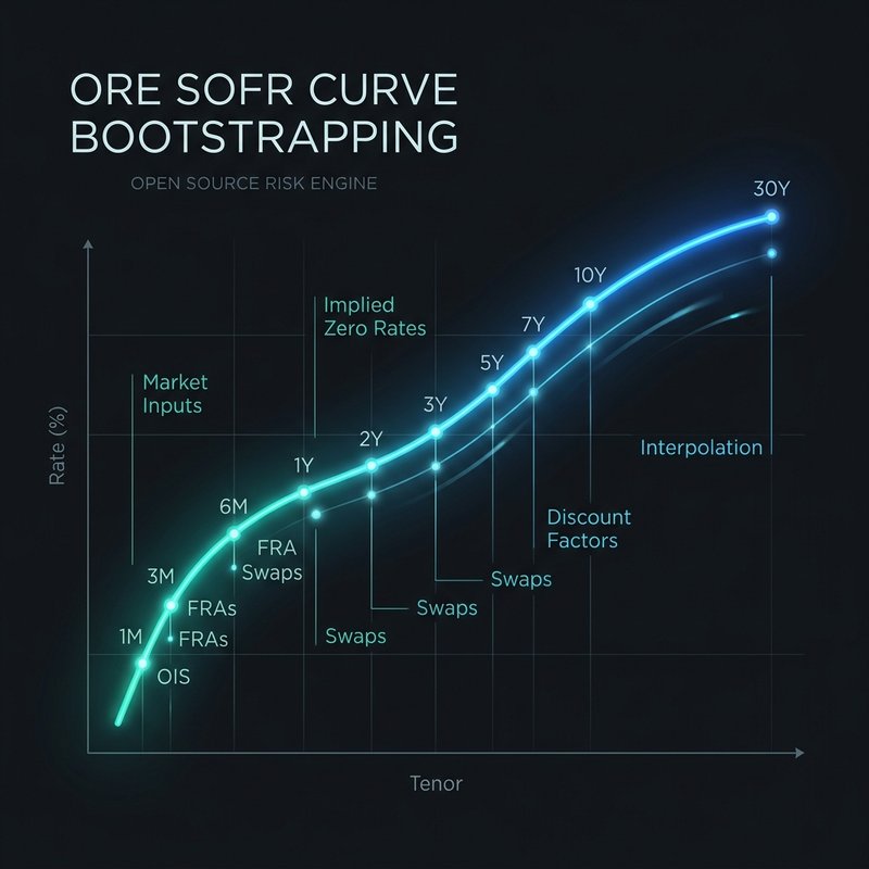
Open Source Risk Engine (ORE) is a powerful, production-grade risk analysis and pricing engine built on top of QuantLib. Having supported multiple clients through vendor replacement processes, we have seen first-hand that interest rate curve bootstrapping is always a critical first step. Reconciling a new open-source library against legacy vendor systems is an iterative, detailed task, and establishing a consistent curve bootstrap is the foundation upon which all downstream valuation and risk metrics depend.
Because ORE is entirely open-source, it offers unmatched transparency for quantitative finance professionals. Rather than dealing with a proprietary “black box”, developers and analysts can inspect every calculation, schedule rule, and day-count convention directly in the source code. A prime example of this transparency is ORE’s official CurveBuilding Examples on GitHub, which showcase how ORE constructs interest rate and inflation curves across different currencies and instruments.
In this post, we pull from these developer examples to walk through how to build a single USD Secured Overnight Financing Rate (SOFR) curve, which acts as both the discounting and forecasting index in the post-LIBOR USD market, and verify the consistency of the bootstrap by repricing the calibration instruments to zero present value (PV).
No C++ compilation is required. You can install the package and run the entire process in a few lines of Python:
pip install open-source-risk-engine matplotlib
1. Mapping the Model — todaysmarket.xml
To understand how ORE resolves your market data, it is helpful to look at the XML config dependency tree. The execution logic flows downward through this hierarchy, making the configuration mapping the natural starting point:
  ore.xml
     │
     └──> todaysmarket.xml
             │
             └──> curveconfig.xml
                     │
                     ├──> conventions.xml
                     └──> market.txt
ore.xml: The master entry point that points ORE to the output directory, logs, portfolio file, and sub-configuration files.todaysmarket.xml: The top-level mapping guide (detailed below). It tells ORE what curves we will build for this run, how to resolve them against configurations incurveconfig.xml, and what curves should be used for discounting and forwarding roles for each currency and index.curveconfig.xml: Defines the recipe for building each individual curve (detailed in Section 4).conventions.xml(detailed in Section 2) +market.txt(detailed in Section 3): Hold the underlying conventions details and numerical rate values.
For our single-curve USD SOFR build, todaysmarket.xml maps both the discounting curve and the index forwarding curve roles to the USD-SOFR curve identifier:
<TodaysMarket>
  <Configuration id="default">
    <DiscountingCurvesId>default</DiscountingCurvesId>
    <IndexForwardingCurvesId>default</IndexForwardingCurvesId>
  </Configuration>
  <DiscountingCurves>
    <DiscountingCurve currency="USD">USD-SOFR</DiscountingCurve>
  </DiscountingCurves>
  <IndexForwardingCurves>
    <IndexForwardingCurve index="USD-SOFR">USD-SOFR</IndexForwardingCurve>
  </IndexForwardingCurves>
</TodaysMarket>
This explicit mapping informs ORE that USD-SOFR is the reference curve for both discounting cashflows and projecting future daily SOFR coupon fixings.
2. Conventions — conventions.xml
Before feeding market quotes to the curve builder, ORE needs to know the financial conventions of the underlying instruments. Every swap coupon payment lag, day count fraction, and business day calendar mismatch will lead to pricing discrepancies if these details are not perfectly specified.
Indeed, a solid understanding of these conventions is key to successful interest rate modelling. For a comprehensive reference on global interest rate market conventions, see the guide by Marc P. A. Henrard: Interest Rate Instruments and Market Conventions Guide - Post LIBOR edition.
For the underlying mathematics of interest rate curve construction, interpolation methods, and multi-curve bootstrapping, the classic paper by Ferdinando M. Ametrano and Marco Bianchetti serves as the reference text: Everything You Always Wanted to Know About Multiple Interest Rate Curve Bootstrapping but Were Afraid to Ask. It is highly recommended reading if you want to dive deep into the bootstrapping mechanics.
For a standard USD SOFR curve build, we combine money market (MM) overnight deposit conventions for the short end and Overnight Indexed Swap (OIS) conventions for the longer tenors. Note, some practitioners would also use SOFR MM Futures as the second component of the bootstrap rather than going directly to OIS Swaps, this is entirely possible in ORE also. The conventions are defined in conventions.xml:
<Conventions>
  <Deposit>
    <Id>USD-ON-SOFR-DEPOSIT</Id>
    <IndexBased>true</IndexBased>
    <Index>USD-SOFR</Index>
  </Deposit>
  <OIS>
    <Id>USD-SOFR-OIS</Id>
    <SpotLag>0</SpotLag>
    <Index>USD-SOFR</Index>
    <FixedDayCounter>A360</FixedDayCounter>
    <PaymentLag>2</PaymentLag>
    <EOM>false</EOM>
    <FixedFrequency>Annual</FixedFrequency>
    <FixedConvention>MF</FixedConvention>
    <FixedPaymentConvention>MF</FixedPaymentConvention>
    <Rule>Backward</Rule>
  </OIS>
</Conventions>
Deconstructing conventions
In ORE, curve conventions are mapped out with fine-grained parameters:
- Overnight Deposit (
USD-ON-SOFR-DEPOSIT): An index-based deposit linking directly to theUSD-SOFRindex. - OIS Conventions (
USD-SOFR-OIS):<SpotLag>: Set to0days, meaning the swap starts immediately on the settlement date.<PaymentLag>: Set to2business days, meaning payments occur 2 days after the accrual period ends.<FixedDayCounter>: Set toA360(Actual/360) day count basis.<FixedConvention>and<FixedPaymentConvention>: Set toMF(Modified Following business day rule).<Rule>: Set toBackwardschedule generation.
3. Market Data — market.txt
Next, we define our market quotes. In a realistic curve build, we start the SOFR curve using the Overnight Money Market (MM) deposit rate helper at the very short end ($T+0$), followed by OIS swaps for the longer tenors. The data is provided in a simple space-delimited text format:
# Node        Instrument Type                    Quote
2023-01-31    MM/RATE/USD/SOFR/0D/1D             0.0430000000
2023-01-31    IR_SWAP/RATE/USD/SOFR/0D/1D/1M     0.0456640000
2023-01-31    IR_SWAP/RATE/USD/SOFR/0D/1D/3M     0.0468210000
2023-01-31    IR_SWAP/RATE/USD/SOFR/0D/1D/6M     0.0483440000
2023-01-31    IR_SWAP/RATE/USD/SOFR/0D/1D/1Y     0.0487100000
2023-01-31    IR_SWAP/RATE/USD/SOFR/0D/1D/2Y     0.0427805000
2023-01-31    IR_SWAP/RATE/USD/SOFR/0D/1D/5Y     0.0346100000
2023-01-31    IR_SWAP/RATE/USD/SOFR/0D/1D/10Y    0.0324600000
2023-01-31    IR_SWAP/RATE/USD/SOFR/0D/1D/30Y    0.0300290000
Quote String Representation & Conventions Control
In ORE, market data quotes follow a structured string format that helps developers identify the instrument type, currency, index, and tenor:
MM/RATE/USD/SOFR/0D/1D: Represents a Money Market (MM) rate for theUSDcurrency, tied toSOFRovernight (starting immediately, term of1D).IR_SWAP/RATE/USD/SOFR/0D/1D/30Y: Represents an Interest Rate Swap (IR_SWAP) rate for theUSDcurrency, tied toSOFRovernight index with a tenor of30Y.
Important: A common point of confusion when setting up ORE is assuming that ORE parses these quote strings to determine pricing behavior. This is not the case.
While the quote string contains parameters like the tenor (
30Y) or settlement terms (0D/1D), the string serves strictly as a key identifier to match the market data row with the curve configuration. The actual financial behavior—such as compounding logic, schedule generation, payment lags, calendars, and rolling conventions—is driven entirely by the conventions defined inconventions.xmlrather than parsed directly from the market data quote string itself.
4. Curve Configuration — curveconfig.xml
With conventions and quotes in hand, we assemble the curve recipe in curveconfig.xml. Because we are using two different types of instruments (a Deposit at the short end and Swaps for the rest of the curve), our configuration defines multiple <Simple> segments:
<CurveConfiguration>
  <YieldCurves>
    <YieldCurve>
      <CurveId>USD-SOFR</CurveId>
      <CurveDescription>USD SOFR OIS discount curve</CurveDescription>
      <Currency>USD</Currency>
      <DiscountCurve>USD-SOFR</DiscountCurve>
      <Segments>
        <Simple>
          <Type>Deposit</Type>
          <Quotes>
            <Quote>MM/RATE/USD/SOFR/0D/1D</Quote>
          </Quotes>
          <Conventions>USD-ON-SOFR-DEPOSIT</Conventions>
          <ProjectionCurve>USD-SOFR</ProjectionCurve>
        </Simple>
        <Simple>
          <Type>OIS</Type>
          <Quotes>
            <Quote optional="true">IR_SWAP/RATE/USD/SOFR/0D/1D/1M</Quote>
            <Quote optional="true">IR_SWAP/RATE/USD/SOFR/0D/1D/3M</Quote>
            <Quote optional="true">IR_SWAP/RATE/USD/SOFR/0D/1D/6M</Quote>
            <Quote optional="true">IR_SWAP/RATE/USD/SOFR/0D/1D/1Y</Quote>
            <Quote optional="true">IR_SWAP/RATE/USD/SOFR/0D/1D/2Y</Quote>
            <Quote optional="true">IR_SWAP/RATE/USD/SOFR/0D/1D/5Y</Quote>
            <Quote optional="true">IR_SWAP/RATE/USD/SOFR/0D/1D/10Y</Quote>
            <Quote optional="true">IR_SWAP/RATE/USD/SOFR/0D/1D/30Y</Quote>
          </Quotes>
          <Conventions>USD-SOFR-OIS</Conventions>
        </Simple>
      </Segments>
      <InterpolationVariable>Discount</InterpolationVariable>
      <InterpolationMethod>LogLinear</InterpolationMethod>
      <YieldCurveDayCounter>A365</YieldCurveDayCounter>
      <Tolerance>0.0000000000010000</Tolerance>
      <Extrapolation>true</Extrapolation>
    </YieldCurve>
  </YieldCurves>
</CurveConfiguration>
Unmatched Control Over Curve Building
One of ORE’s core strengths is the level of mathematical control it gives you over the curve construction process. Rather than restricting you to a single hard-coded solver, ORE exposes configuration fields for every stage of the interpolation and bootstrapping math:
A. Interpolation Variables
You can choose the domain on which interpolation is performed (<InterpolationVariable>):
Discount(Default): Interpolates discount factors directly.Zero: Interpolates continuously compounded zero rates.Forward: Interpolates instantaneous forward rates.
B. Interpolation Methods
ORE supports a wide variety of interpolation algorithms (<InterpolationMethod>), letting you select the method that best aligns with your risk and pricing needs:
Linear/LogLinear: Simple and robust.LogLinearinterpolation onDiscountfactors is equivalent to assuming piecewise-constant forward rates (flat forwards)—a standard market choice.NaturalCubic/FinancialCubic: Smoother cubic spline variants.FinancialCubicensures zero second derivative at the left edge and zero first derivative at the right edge.ConvexMonotone: Hagan & West’s method, designed to preserve convexity and monotonicity of forward rates.LogNaturalCubic/LogFinancialCubic/LogCubicSpline: Cubic splines applied in the natural log domain of the target variable.BackwardFlat: Piecewise constant, right-continuous interpolation.
C. Handling the $t_0$ Reference Date
The optional <ExcludeT0FromInterpolation> element (set to True or False) lets you exclude the synthetic time-zero ($t_0$) reference point (where $DF=1.0$) from the interpolation grid. When set to True, the curve interpolates strictly on actual market pillar dates, using flat zero/forward rates between $t_0$ and the first pillar. This avoids forcing a synthetic anchor point that can distort the short end of the curve.
D. Bootstrapping Precision & Performance
Under the optional <BootstrapConfig> node, ORE exposes parameters for the iterative root-finding procedure:
<Accuracy>(Default:1e-12): The desired tolerance for the root-finding solver to match market quotes.<GlobalAccuracy>: Tolerable fallback accuracy if target accuracy cannot be met.<DontThrow>: If set toTrue, ORE will continue execution using the best fit found rather than throwing an exception if the global accuracy check fails.<MaxAttempts>(Default:5): Maximum attempts/seed trials for fitting complex curves (like Fitted Bond curves using Nelson-Siegel or Svensson methods).<ExtrapolationMethod>: Controls curve tails usingContinuousForward(flat instantaneous forwards) orDiscreteForward(flat daily forwards).
5. Bootstrapping and Plotting in Python
We can execute the entire calibration run and extract the zero rates directly in a Python script. ORE reads our master execution config (ore.xml) and calibrates the curve.
Here is the Python script to run the bootstrapping and plot the zero curve:
import os
import ORE as ore
import csv
import matplotlib.pyplot as plt
from pathlib import Path

# Set up base path relative to this script
BASE_DIR = Path(__file__).parent.resolve()
INPUT_DIR = BASE_DIR / "Input"
OUTPUT_DIR = BASE_DIR / "Output"

os.makedirs(OUTPUT_DIR, exist_ok=True)

# 1. Run the ORE App
params = ore.Parameters()
params.fromFile(str(INPUT_DIR / "ore.xml"))
app = ore.OREApp(params)
app.run()

print("\n--- ORE Run Completed Successfully ---\n")

# 2. Extract bootstrapped curve rates
analytic = app.getAnalytic("NPV")
market = analytic.getMarket()
curve = market.discountCurve("USD")

tenors = {
    "1M": 1/12,
    "3M": 0.25,
    "6M": 0.5,
    "1Y": 1.0,
    "2Y": 2.0,
    "5Y": 5.0,
    "10Y": 10.0,
    "30Y": 30.0
}

times = []
zero_rates = []

print("Discount Factors and Zero Rates (as of 2023-01-31):")
print(f"{'Tenor':<8} {'Time (y)':<10} {'Discount Factor':<18} {'Zero Rate (%)':<15}")
print("-" * 55)

for name, t in tenors.items():
    df = curve.discount(t)
    zero = curve.zeroRate(t, ore.Compounded, ore.Annual).rate()
    times.append(t)
    zero_rates.append(zero * 100)
    print(f"{name:<8} {t:<10.4f} {df:<18.8f} {zero*100:<15.4f}%")

# 3. Plot the zero curve
fig, ax = plt.subplots(figsize=(10, 5))
ax.plot(times, zero_rates, marker="o", linewidth=2, color="steelblue", label="USD SOFR Zero Rate")
ax.set_xlabel("Time (years)")
ax.set_ylabel("Zero Rate (%)")
ax.set_title("Bootstrapped USD SOFR Zero Curve (As of 2023-01-31)")
ax.legend()
ax.grid(True, linestyle="--", alpha=0.5)
plt.tight_layout()
plt.savefig("zero_curve.png", dpi=150)
plt.show()
print("Zero curve saved to zero_curve.png")
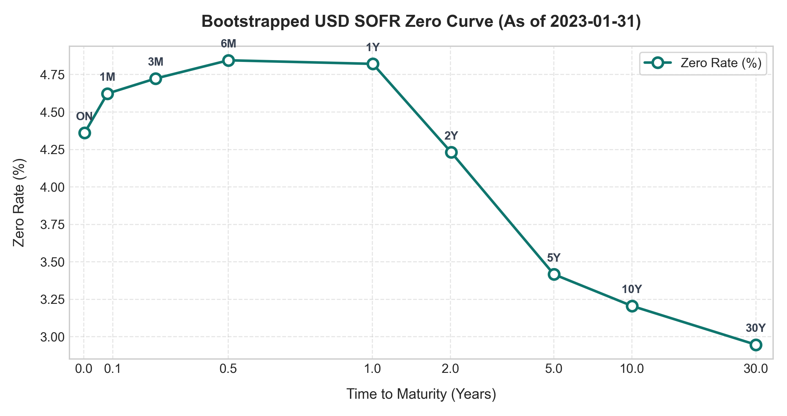
When we run this script, we obtain the zero-rate curve plot shown below:
6. Under the Hood: ORE Calibration Reports
One of the most powerful features added in recent ORE releases is the automatic generation of detailed calibration reports. In the execution output, you will find todaysmarketcalibration.csv and todaysmarketcalibration_cashflows.csv under the Output directory.
For anyone trying to understand the mechanics of the bootstrap, todaysmarketcalibration_cashflows.csv is an absolute goldmine.
Instead of treating the bootstrap as a black-box mathematical solver, ORE writes out the complete cashflow schedule of every rate helper instrument utilized in the curve calibration. For each instrument (e.g., our USD SOFR OIS swaps), the report details:
- Pillar Dates and Accrual Start/End Dates.
- Projected Interest Amounts and Accrual Fractions.
- Fixing Dates and Forward Rate Fixing Values.
- Discount Factors and Present Values (PV) of both legs.
Having direct visibility into these details significantly speeds up the implementation and debugging process. Day-count fraction errors or payment lag mismatches become instantly noticeable as you inspect the exact schedules and discount factors used.
To see this in action, here is an extract of the cashflows for the 2Y OIS Swap (market fixed quote: 4.27805%) from the report. It shows how the Fixed and Floating legs are structured:
| Leg | Pay Date | Accrual Start | Accrual End | Accrual Fraction | Rate (%) | Discount Factor | Present Value (USD) |
|---|---|---|---|---|---|---|---|
| Fixed | 2024-02-02 | 2023-01-31 | 2024-01-31 | 1.013889 | 4.27805% | 0.952687 | 41,322.50 |
| Fixed | 2025-02-04 | 2024-01-31 | 2025-01-31 | 1.016667 | 4.27805% | 0.918343 | 39,941.96 |
| Floating ¹ | 2024-02-02 | 2023-01-31 | 2024-01-31 | 1.013889 | 4.87100% | 0.952687 | -47,049.92 |
| Floating ¹ | 2025-02-04 | 2024-01-31 | 2025-01-31 | 1.016667 | 3.66461% | 0.918343 | -34,214.54 |
¹ On an OIS floating leg, no single overnight rate is fixed in advance. Instead, the daily SOFR fixings are compounded over each accrual period. The rates shown above (4.87100% for Period 1 and 3.66461% for Period 2) are the equivalent flat rate that would produce the same compounded interest amount over the period—sometimes called the projected par coupon rate. Period 1’s rate exactly matches the 1Y market quote (4.871%), which makes sense: the 1Y OIS calibration instrument was already bootstrapped, and its projected compounded rate is the 1Y fair rate. Period 2’s rate (3.665%) is what the bootstrapper must solve for to make the 2Y swap price at par.
Summing the present values:
- Fixed Leg PV: $+81,264.46$ USD
- Floating Leg PV: $-81,264.46$ USD
- Net Swap NPV: $0.00$ USD
This demonstrates the mathematical core of the bootstrap: the solver finds the equivalent compounded forward rate for the second period (3.66461%) such that the floating leg PV exactly matches the fixed leg PV.
7. From Conventions to Dates — A Worked Example
The cashflow report above is where we can see the exact output of ORE’s date math. Rather than being magic numbers, every single date and accrual fraction here is a direct, deterministic consequence of the as-of date, the instrument tenor, and the conventions.
For our 2Y USD SOFR swap, ORE picks up the conventions from the <Conventions>USD-SOFR-OIS</Conventions> node in curveconfig.xml. This refers back to the matching <OIS> convention block in conventions.xml containing SpotLag, PaymentLag, FixedDayCounter, Rule, etc.
Here is how ORE resolves the dates step-by-step for the 2Y instrument:
Step 1 — Determine the Start Date (SpotLag = 0)
Our market data as-of date is 2023-01-31. Since <SpotLag> is set to 0, there is no settlement delay. The swap starts immediately on the trade date:
$$\text{Start Date} = \text{2023-01-31} + 0 \ \text{business days} = \textbf{2023-01-31}$$
Step 2 — Determine the End Date (Tenor = 2Y)
Adding the 2Y tenor to our start date gives the unadjusted end date:
$$\text{Unadjusted End} = \text{2023-01-31} + 2Y = \text{2025-01-31}$$
Since January 31, 2025 is a Friday (a valid business day), no business day adjustment is needed. The maturity date is 2025-01-31.
Step 3 — Generate the Schedule (Rule = Backward)
Because the schedule rule is set to Backward, ORE builds the schedule by stepping back from the maturity date in annual increments (based on <FixedFrequency>Annual</FixedFrequency>):
| Step | Date | Adjustment | Result |
|---|---|---|---|
| Maturity | 2025-01-31 | — | 2025-01-31 |
| −1Y | 2024-01-31 | Valid business day | 2024-01-31 |
| −2Y | 2023-01-31 | Valid business day (= Start) | 2023-01-31 |
This gives us two accrual periods:
- Period 1:
2023-01-31to2024-01-31 - Period 2:
2024-01-31to2025-01-31
Step 4 — Calculate Payment Dates (PaymentLag = 2)
Payments are made 2 business days after the end of each accrual period, adjusted using the Modified Following (MF) business day convention:
| Accrual End | +2 bd | Payment Date |
|---|---|---|
| 2024-01-31 (Wed) | → 2024-02-01 (Thu) → 2024-02-02 (Fri) | 2024-02-02 ✓ |
| 2025-01-31 (Fri) | → 2025-02-03 (Mon) → 2025-02-04 (Tue) | 2025-02-04 ✓ |
These dates match the PayDate values in our cashflow report exactly.
Step 5 — Calculate Accrual Fractions (FixedDayCounter = A360)
Using the Actual/360 convention, we divide the actual number of calendar days in the period by 360:
| Period | Start | End | Actual Days | Fraction (days/360) |
|---|---|---|---|---|
| 1 | 2023-01-31 | 2024-01-31 | 365 | $365 / 360 = \mathbf{1.013889}$ ✓ |
| 2 | 2024-01-31 | 2025-01-31 | 366 | $366 / 360 = \mathbf{1.016667}$ ✓ |
Note that 2024 is a leap year, so the second period contains 366 calendar days, yielding the slightly larger accrual fraction seen in the report.
Step 6 — Calculate the Fixed Coupon Amount
With a fixed rate of 4.27805% and a $1,000,000 notional, the coupon for the first period is:
$$\text{Coupon}_1 = 1{,}000{,}000 \times 0.0427805 \times 1.013889 = \mathbf{$43{,}374.67}\text{ USD}$$
Discounting this cashflow with the bootstrapped 1Y discount factor of 0.952687 gives:
$$\text{PV}_1 = 43{,}374.67 \times 0.952687 = \mathbf{$41{,}322.50}\text{ USD}$$
Both figures reconcile perfectly with the values in the ORE calibration report. Everything falls out cleanly from just a few parameters: the start date, the tenor, spot lag, frequency, payment lag, and day count convention.
8. Verification — The Zero-PV Repricing Check
A successful bootstrap means that the constructed curve must perfectly replicate the market prices of the instruments used to build it. To prove this, we construct a portfolio of matching OIS swaps in portfolio.xml (e.g., matching the 1M, 1Y, and 5Y points with the respective market fixed rates) and price them against our newly constructed curve:
<Portfolio>
  <Trade id="OIS_5Y">
    <TradeType>Swap</TradeType>
    <Envelope>
      <CounterParty>CPTY_A</CounterParty>
      <NettingSetId>CPTY_A</NettingSetId>
      <AdditionalFields/>
    </Envelope>
    <SwapData>
      <LegData>
        <LegType>Fixed</LegType>
        <Payer>false</Payer>
        <Currency>USD</Currency>
        <Notionals><Notional>10000000</Notional></Notionals>
        <DayCounter>A360</DayCounter>
        <PaymentConvention>ModifiedFollowing</PaymentConvention>
        <PaymentLag>2</PaymentLag>
        <FixedLegData><Rates><Rate>0.034610</Rate></Rates></FixedLegData>
        <ScheduleData>
          <Rules>
            <StartDate>2023-01-31</StartDate>
            <EndDate>2028-01-31</EndDate>
            <Tenor>1Y</Tenor>
            <Calendar>US</Calendar>
            <Convention>ModifiedFollowing</Convention>
            <TermConvention>ModifiedFollowing</TermConvention>
            <Rule>Backward</Rule>
          </Rules>
        </ScheduleData>
      </LegData>
      <LegData>
        <LegType>Floating</LegType>
        <Payer>true</Payer>
        <Currency>USD</Currency>
        <Notionals><Notional>10000000</Notional></Notionals>
        <DayCounter>A360</DayCounter>
        <PaymentLag>2</PaymentLag>
        <PaymentConvention>ModifiedFollowing</PaymentConvention>
        <FloatingLegData>
          <Index>USD-SOFR</Index>
        </FloatingLegData>
        <ScheduleData>
          <Rules>
            <StartDate>2023-01-31</StartDate>
            <EndDate>2028-01-31</EndDate>
            <Tenor>1Y</Tenor>
            <Calendar>US</Calendar>
            <Convention>ModifiedFollowing</Convention>
            <TermConvention>ModifiedFollowing</TermConvention>
            <Rule>Backward</Rule>
          </Rules>
        </ScheduleData>
      </LegData>
    </SwapData>
  </Trade>
</Portfolio>
When ORE prices these trades using the bootstrapped curve, the output reports NPVs of exactly 0.000000:
| Trade ID | Leg 1 Type | Leg 2 Type | Notional (USD) | NPV (USD) | Base NPV (USD) |
|---|---|---|---|---|---|
| OIS_1M | Fixed | Floating | 10,000,000.00 | 0.000000 | 0.000000 |
| OIS_1Y | Fixed | Floating | 10,000,000.00 | 0.000000 | 0.000000 |
| OIS_5Y | Fixed | Floating | 10,000,000.00 | 0.000000 | 0.000000 |
This confirms that our bootstrapping configuration is consistent and perfectly reproduces the input market quotes.
9. Sanity Check — Breaking the Linkage
To demonstrate that our zero-PV result is a meaningful validation of the bootstrap rather than a configuration triviality, we can introduce a deliberate mismatch. If we perturb one of the swap fixed rates in our portfolio to 3.561% (+10 bps) without rebuilding the curve, and re-price:
| Trade ID | NPV (USD) | Base NPV (USD) |
|---|---|---|
| OIS_5Y | 45,379.995138 | 45,379.995138 |
The NPV deviates significantly from zero. This demonstrates that the zero-PV check is highly sensitive to the exact alignment between the curve calibration quotes and the trade valuation models.
10. Testing ORE Against Your Existing System
If you are looking to integrate ORE into your workflow, the best way to start is by testing it against your current library or legacy pricing system. This is typically an iterative process:
- Align on Conventions & Market Data: Ensure your day-count conventions, calendar adjustment rules, holiday calendars, spot lags, and market rate inputs (in
market.txt) are exactly identical to your current system. - Replicate the Curve Configuration: Re-create the interpolation method (e.g., LogLinear discount factor interpolation) and segment definitions.
- Compare Discount Factors: Calibrate the curves in both systems for the same as-of date and compare the resulting discount factors at various tenors.
Discrepancies during this comparison are common and usually trace back to subtle differences in schedule rules or accrual fraction calculations. This is where ORE’s new todaysmarketcalibration_cashflows.csv report becomes invaluable. By comparing ORE’s detailed cashflow schedule and discount factors side-by-side with vendor libraries, you can pinpoint the exact payment date or compounding difference causing the divergence, drastically reducing integration time.
By following this disciplined comparison, you can gain high confidence in ORE’s open-source calculations. But establishing a solid, verified bootstrap is just the first step. Once you have matching curves, you unlock the ability to leverage ORE’s wider ecosystem for full portfolio valuation, XVA, historical simulation, and market risk analytics. Reconciling your curves is the ideal foundation for a much broader ORE integration journey.
Source Code
All configuration files and the Python script used in this post are available for download: Download Source Code
Disclaimer: The minimal ORE inputs utilized in this post, along with the featured graphics, were generated and coordinated using Gemini 3.5 Flash and Nano Banana 2.

Joey O'Brien
Principal Consultant
Principal Consultant in the Quant Services division of LSEG, specializing in model validation, derivative pricing, and risk solutions.